Project 1: Colorizing the Prokudin-Gorskii photo collection (GitHub repo)
1. Background
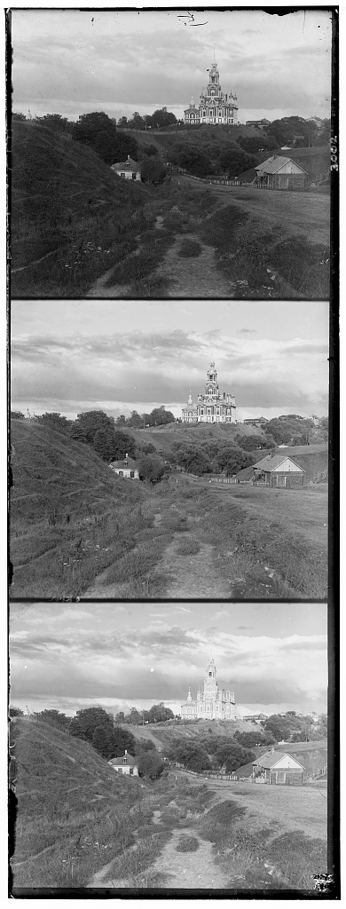
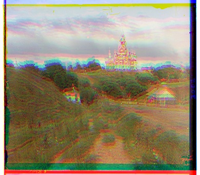
Sergei Mikhailovich Prokudin-Gorskii's photo collection consists of images where three separate exposures of a scene were captured on a glass plate using red, green, and blue filters (allowing only red, green, and blue light to pass through). To produce high-quality colorized photos, a key challenge is properly aligning these three color channels. The objective of this project is to develop a method for aligning the photos from these channels to create a high-quality color image.
2. Implementation
2.1 Single Scale
One proposed pipeline is shown as follows:

The main work here is to develop the Find alignment method. The rest part were implemented as follows:
- Crop photo: For now it simply cut the photos at its 1/3 and 2/3 height.
- Align photos: I used OpenCV's
warpAffinefunction to shift the images by the estimated displacement. - Map to color: One-to-one mapping from three color-filtered channel to RGB value. I
used
numpy.dstackto stack the three channel's pixel value to colorize the photos.
To find the optimal photo alignment, a simple approach is to use a brute-force search within an
alignment window (e.g., [-15, 15] pixels around the initial alignment value). The goal is to
identify the alignment that minimizes a defined cost function. In this project, I used the
Euclidean distance between the two images as the cost function, calculated as
sqrt(sum(image1-image2)^2). For better performance, I utilized numpy.linalg.norm.
Before computing the cost, I adopted two pre-processing strategies:
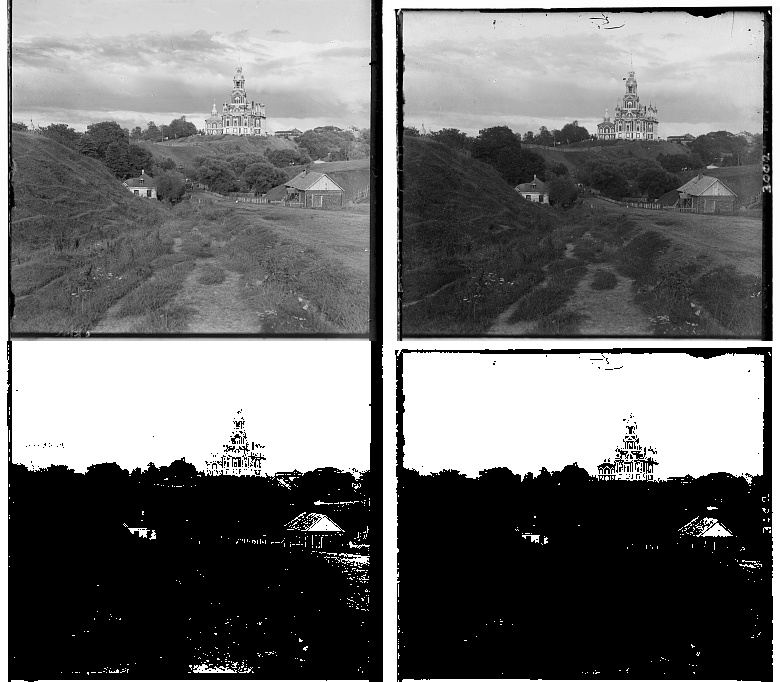
- Photo binarization: I experimented with several methods and found that converting the images to black and white improves the alignment results. This is likely because black and white conversion helps to remove noise and simplifies the image by focusing on areas with strong contrast. I used a threshold of 0.5 for one fixed channel (e.g., the green channel photo) and computed the threshold for the other photo based on their mean pixel value ratio. While more sophisticated binarization methods, such as the [Otsu method], are available, this approach is simple and sufficient for the current project.
- Remove photo margins: The black and white borders of the photos can affect the cost function and reduce alignment quality. To mitigate this, I computed the overlap region of the two images using only 2/3 of the input image, excluding the margins. This also reduces the number of compared pixels and speeds up the process.
2.2 Multi-scale Pyramid
For high-resolution photos, brute-force search is time-consuming; therefore, I adopted the multi-scale pyramid method. The pipeline is shown as follows:

There are two new elements:
resize method (a larger N value means the image is coarser.).
Note that while the user can specify the maximum
scale of the pyramid, experiments indicated that overly downsampled photos can harm the
alignment result. Therefore, this method should prevent resizing photos below a certain
threshold. 2.3 Pseudocode
Below is the pseudocode for finding image alignment, including both single-scale and multi-scale approaches, as well as the image pyramid method. You can find the python implementation here.
                            function findAlignmentSingleScale(image1, image2, initial_dx, initial_dy, search_window):
                                // normalize images
                                image1 <- normalize(image1)
                                image2 <- normalize(image2)

                                // set binarization threshold
                                threshold2 <- 0.5
                                threshold1 <- threshold2 * (mean(image1) / mean(image2))

                                // binarize images
                                image1 <- binarization(image1, threshold1)
                                image2 <- binarization(image2, threshold2)

                                // brute-force serach
                                best_dx <- dx
                                bext_dy <- dy
                                best_cost <- M
                                for dx in initial_dx+search_window
                                    for dy in initial_dy+search_window
                                        image1, image2 <- find_overlap_region(image1, image2, dx, dy)
                                        image1, image2 <- remove_margin(image1, image2, margin_offset)
                                        cost <- Euclidean_distance(image1,image2)
                                        if cost < best_cost
                                            best_dx <- dx
                                            best_dy <- dy

                                return best_dx, best_dy


                            function findAlignmentMultiScale(pyramid1, pyramid2, scale, initial_dx, initial_dy, search_window):
                                // recursion guard
                                if scale < 0:
                                    return initial_dx, initial_dy

                                // retrive images at the current scale from the pyramids
                                image1 <- pyramid1[scale]
                                image2 <- pyramid2[scale]

                                // find best alignment at the current scale
                                best_dx, best_dy <- findAlignmentSingleScale(image1, image2, initial_dx, initial_dy, search_window)

                                // recursive call for the next scale (higher resolution)
                                scale <- scale-1
                                return findAlignmentMultiScale(pyramid1,pyramid2,scale, best_dx, best_dy, search_window)


                            function createImagePyramid(image, max_scale):
                                pyramid <- Empty List
                                // Compute the mathematically available maximum scale
                                max_scale <- min(log2(image_width), log2(image_height), max_scale)

                                for scale in range(max_scale):
                                    // Compute new image size
                                    new_width <- image_width / pow(2, scale)
                                    new_height <- image_height / pow(2, scale)

                                    // Prevent overly downsampled image
                                    if new_width < size_threshold or new_height < size_threshold:
                                        return pyramid

                                    // Resize image to new dimensions
                                    new_image <- resize_image(image, new_width, new_height)
                                    pyramid.add(new_image)

                                return pyramid
Improvement
To enhance the image quality, two improvement has been made.
Color mapping
Up until now, I have directly mapped the red, green, and blue filtered photos to their corresponding RGB channels. However, this might not result in the "correct" mapping that gives a "modern" color photo appearance. To make the coloring closer to modern photos, I assume there is a linear transformation that maps the filtered photo values to RGB values, and this transformation remains consistent across all photo collections, as long as the hardware does not change.
The "correct" RGB color can be express as a 3x1 column vector b and the original color is a 3x1 column vector x, and our goal is to find such a 3x3 transformation matrix A such that Ax=b.
To solve the linear system, we need at least three pairs of x and b. The original system can be expanded as A[x1, x2, ..., xn] = [b1, b2, ..., bn], where n ≥ 3. To obtain the color pairs, I used color-picking tools to select colors from representative objects (e.g., the color of the sky, trees, clothes) and matched them with colors from similar objects in modern photos. Since pixel-level color picking and pairing may not be entirely accurate and can easily introduce bias and outliers, it would be better to have a larger set of color pairs. For this project, due to time constraints, I used six color pairs to compute the transformation matrix. Although the result is not perfect, it does help reduce some of the bluish tint in the photos.
Automatic Image Border Cropping
As you can see in the results section, there are black, white, and other colored margins around the photo borders. To automatically detect and remove them, I tested several strategies, and I will present the one that I believe is (currently) the most stable. The proposed pipeline is as follows:

The overall idea is to compute a cost function based on the differences between pixel vectors in rows or columns. If the cost satisfies certain conditions, the current row or column is considered part of the border. The cost function used here is simply the L2 norm, and the stopping criteria are based on predefined thresholds for the L2 norm and the standard deviation of pixel values in the current row or column. The search starts at the center and moves toward the four borders. To speed up the process, I assume the border is near the edge of the photo, so the search begins close to the edge and this is a reasonable assumption. A row or column is only considered part of the border if its cost is below the threshold (indicating neighboring rows/columns have similar colors) and its standard deviation is below the threshold (indicating uniform color).
There are a few assumptions to consider: the border should have some thickness (i.e., 'width' ≥ 2 pixels) and a uniform color (i.e., small standard deviation in pixel values along the same border). Furthermore, I assume there is no uniform color across the entire photo (e.g., no green screen background). These assumptions ensure that only the border satisfies these conditions.
Result
Below are the results from the sample data. The displacement vectors/alignment vectors are referenced to the top-left corner of the green channel photo. One the left side are the aligned and colorized photos and on the right side are the improved (color remapped and after border cropping) photos.
Low resolution images
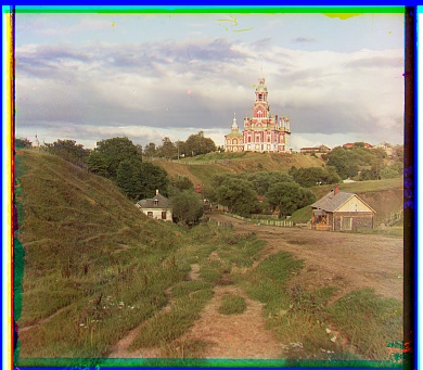
Displacement vectors (dx,dy): r:[2,5], b:[3,12]
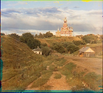
Displacement vectors (dx,dy): r:[2,5], b:[3,12]
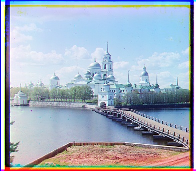
Displacement vectors (dx,dy): r:[2,-3], b:[2,3]
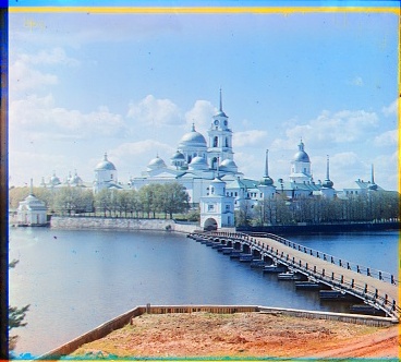
Displacement vectors (dx,dy): r:[2,-3], b:[2,3]
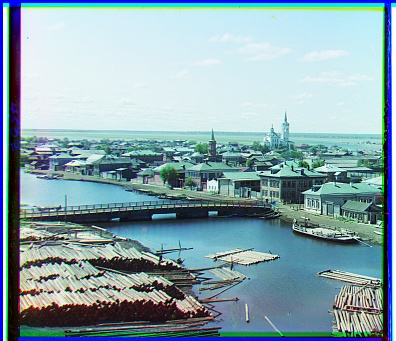
Displacement vectors (dx,dy): r:[3,-3], b:[3,7]
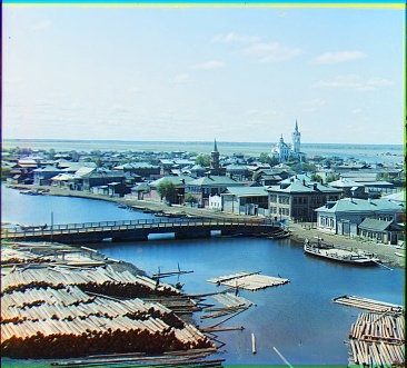
Displacement vectors (dx,dy): r:[3,-3], b:[3,7]
High resolution images
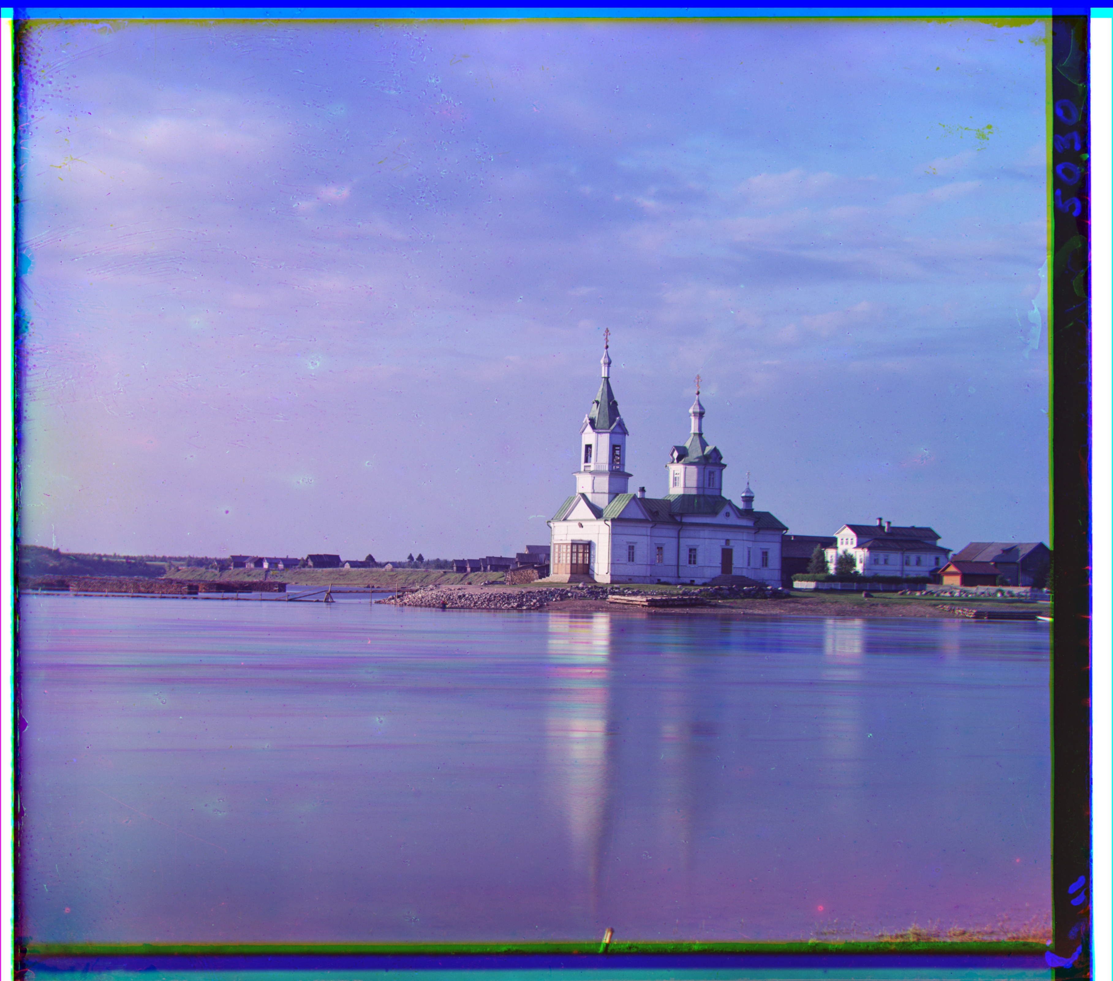
Displacement vectors (dx,dy): r:[3,25], b:[-4,58]
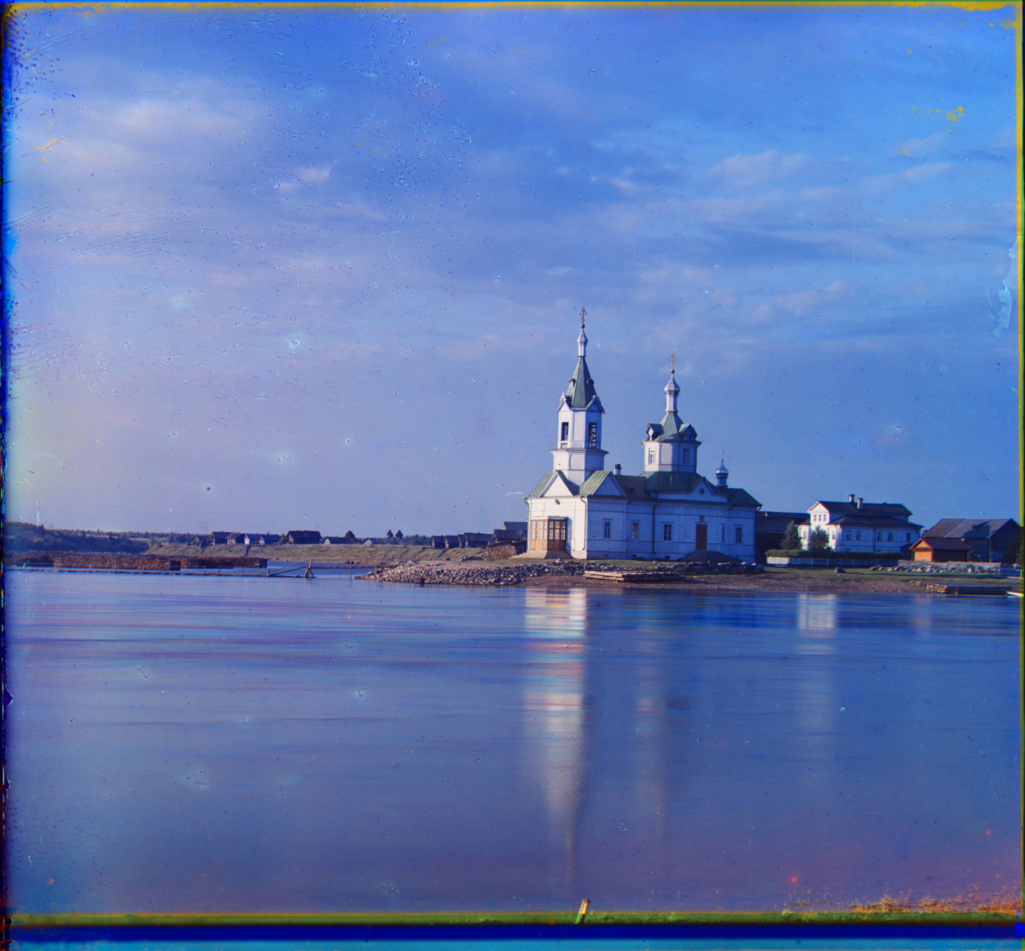
Displacement vectors (dx,dy): r:[3,25], b:[-4,58]
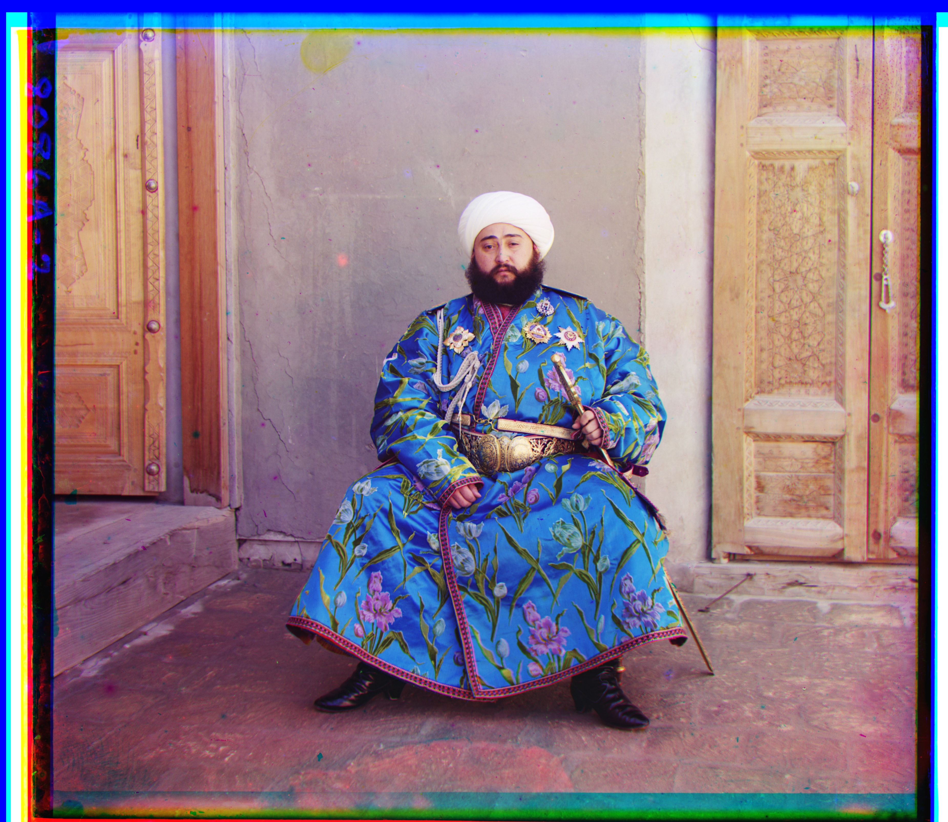
Displacement vectors (dx,dy): r:[24,48], b:[42,105]
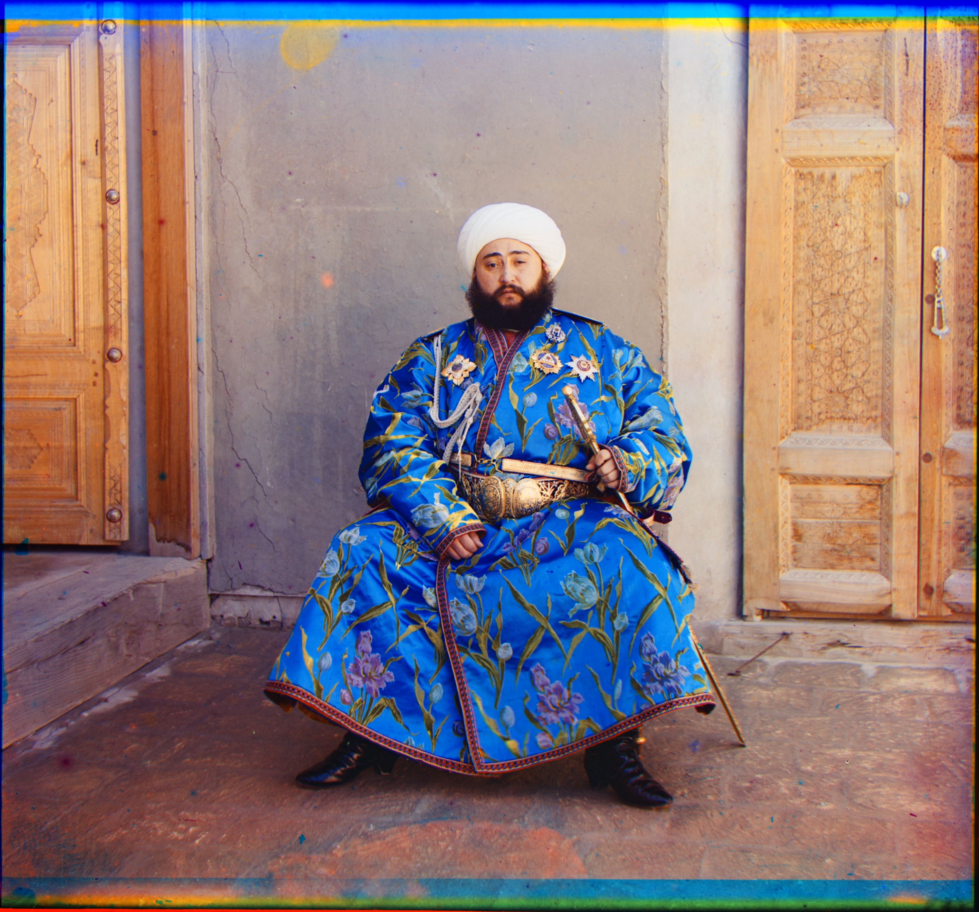
Displacement vectors (dx,dy): r:[24,48], b:[42,105]
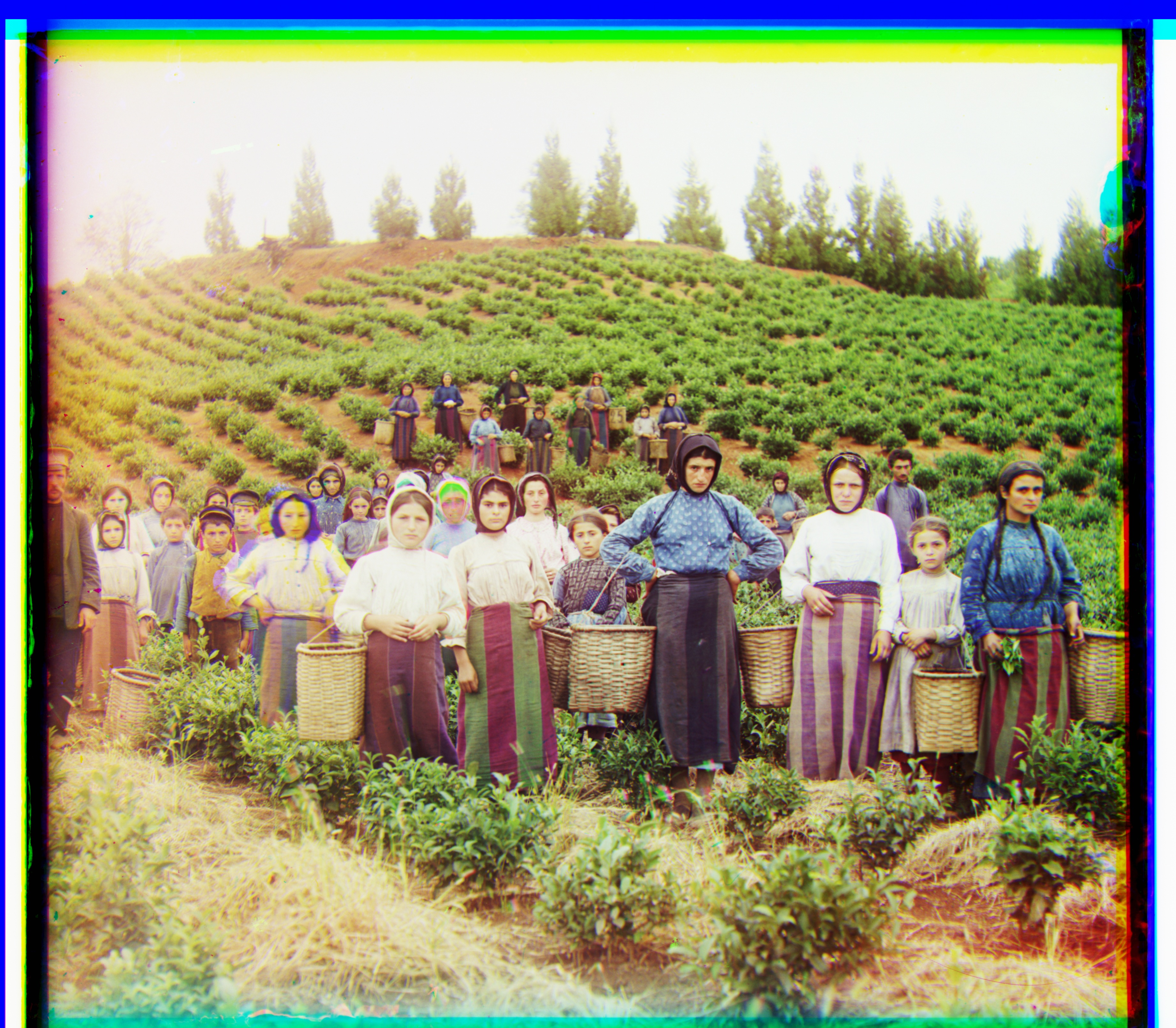
Displacement vectors (dx,dy): r:[17,60], b:[15,124]
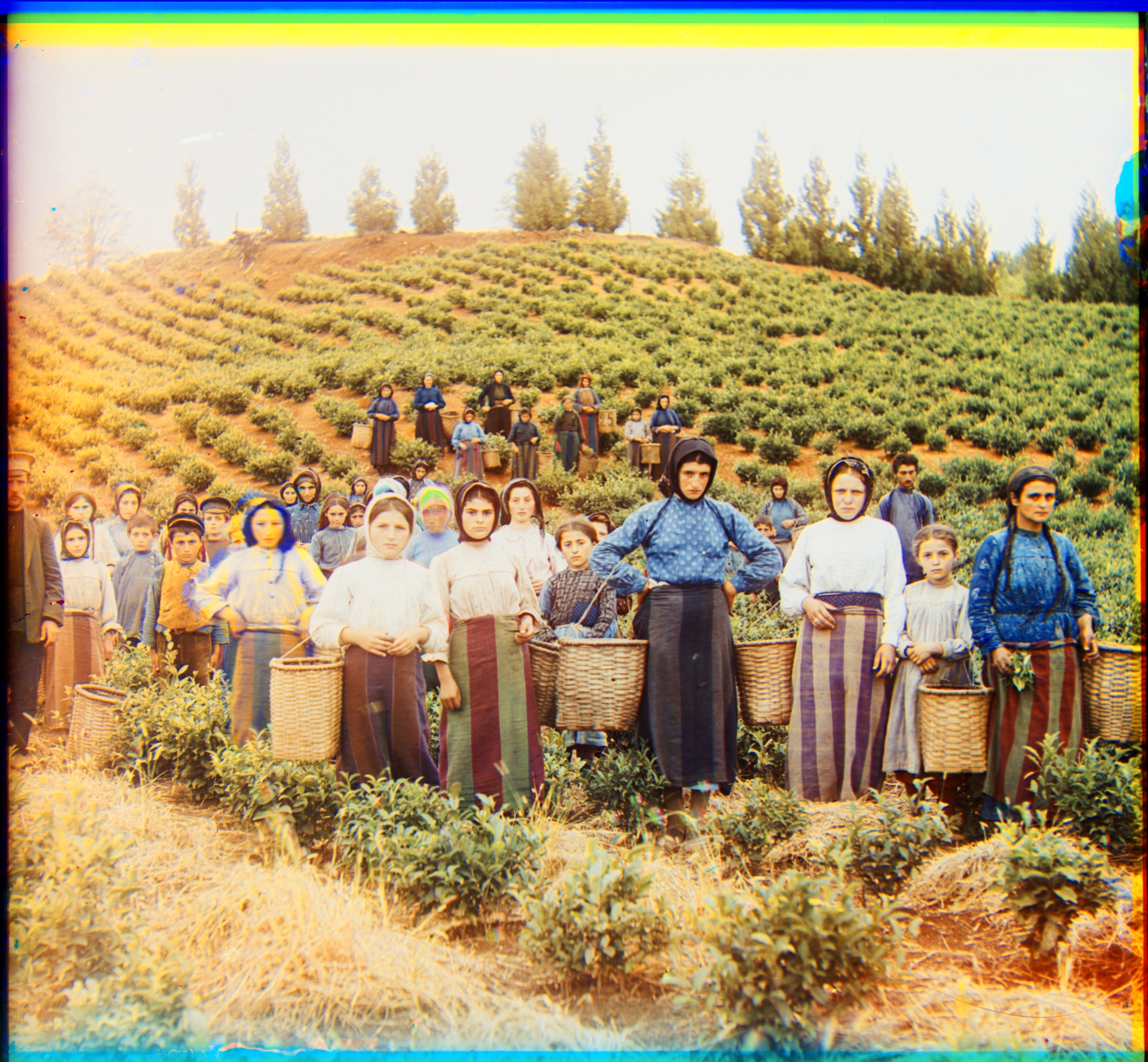
Displacement vectors (dx,dy): r:[17,60], b:[15,124]
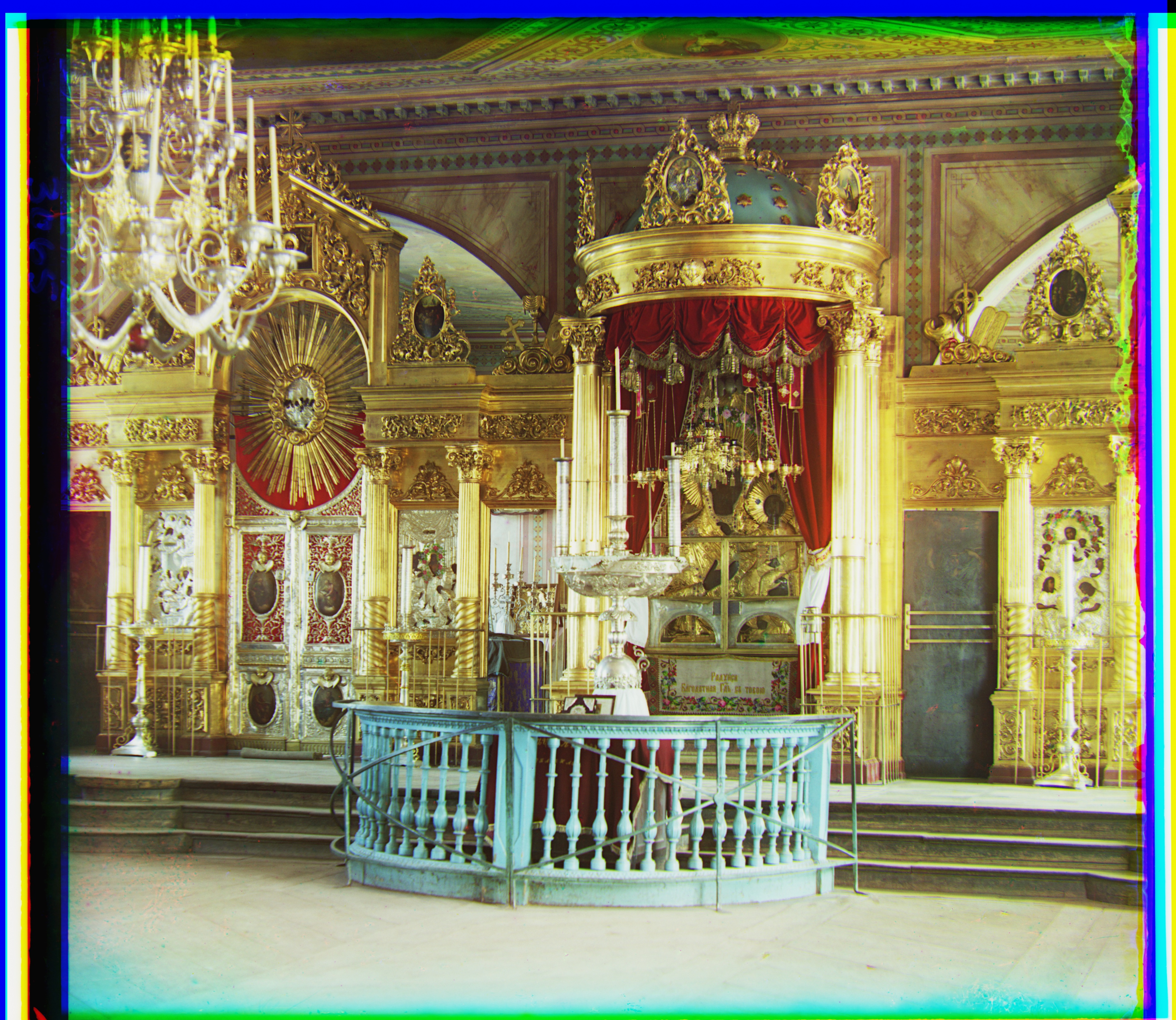
Displacement vectors (dx,dy): r:[17,41], b:[23,90]
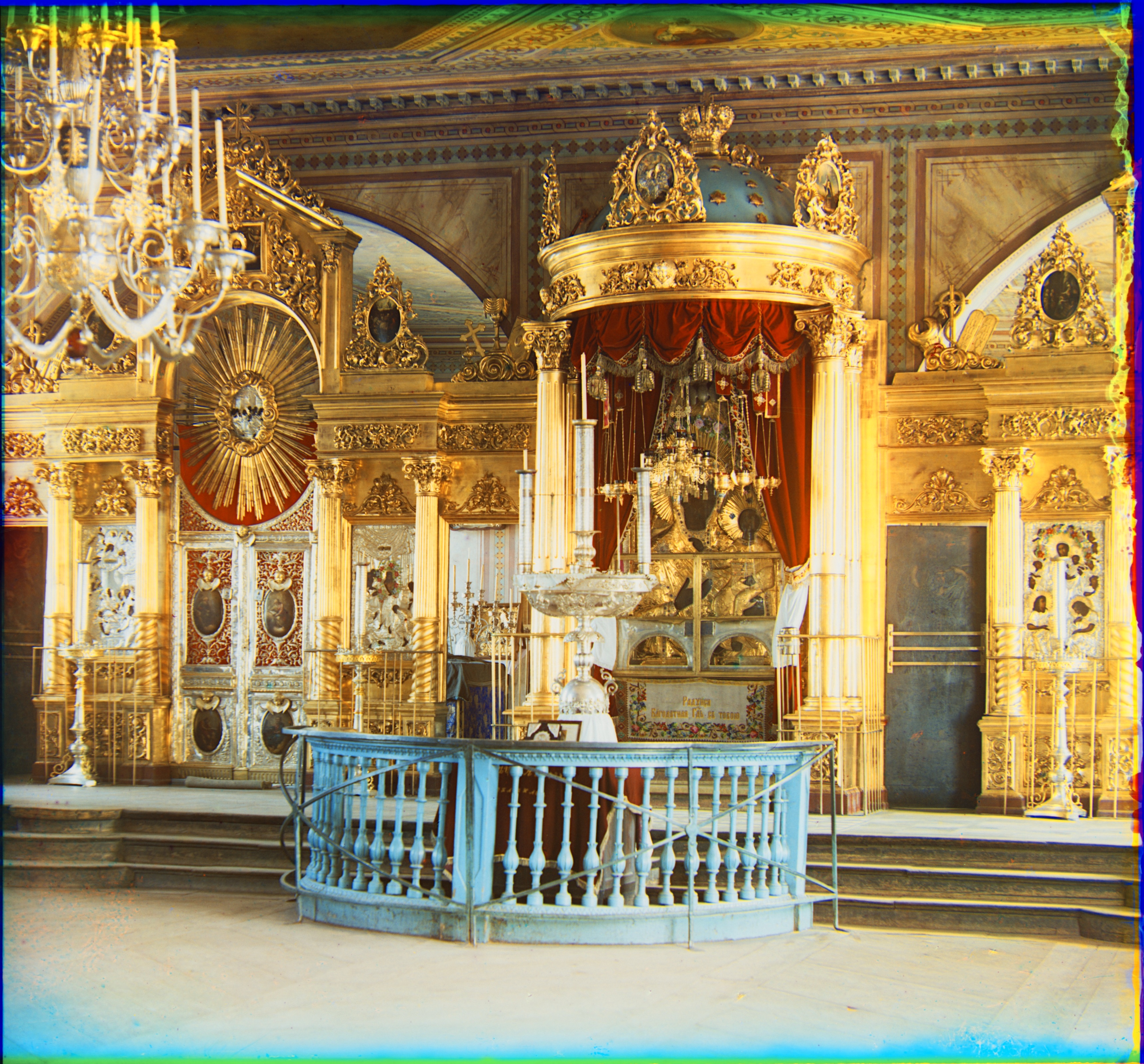
Displacement vectors (dx,dy): r:[17,41], b:[23,90]
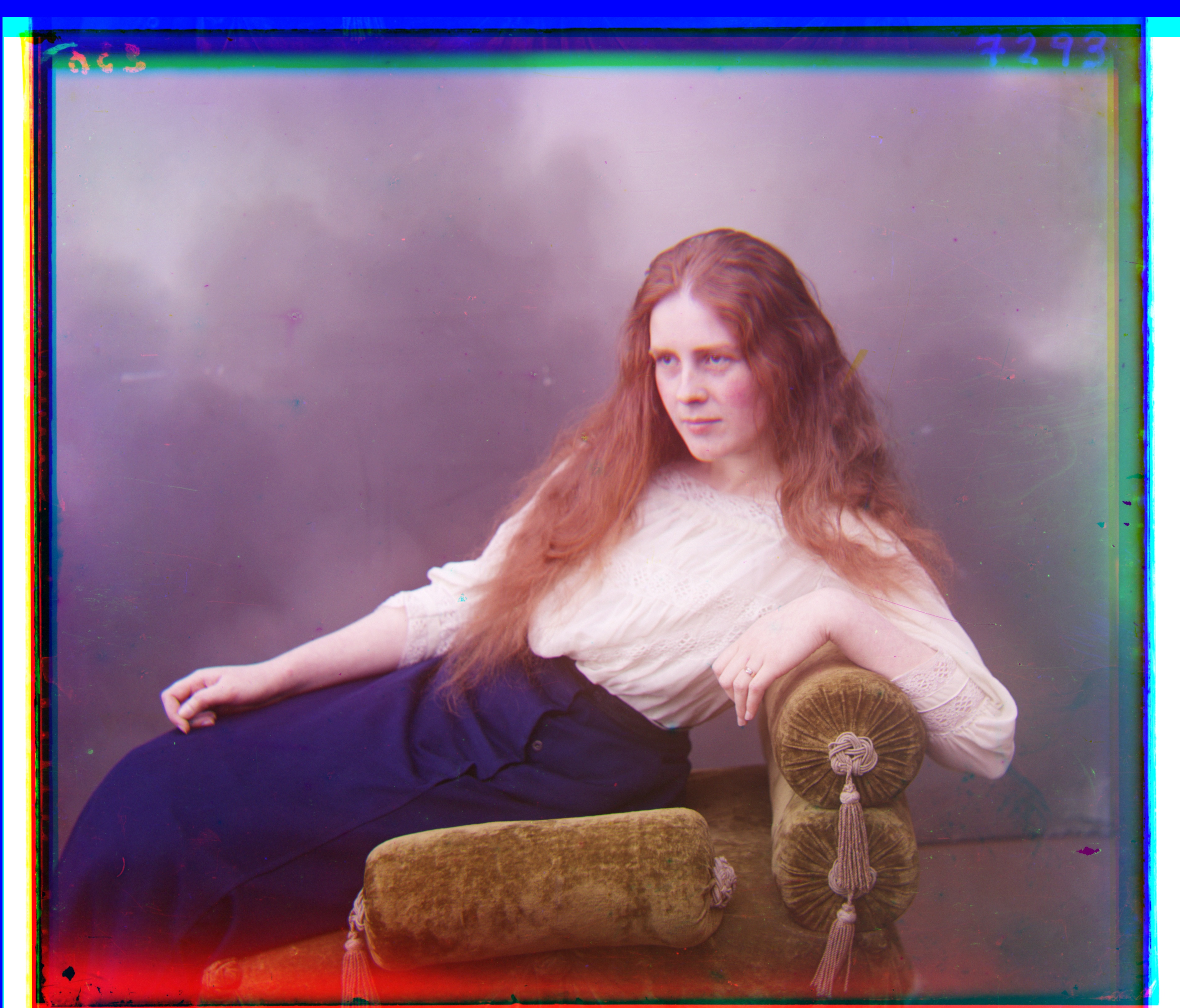
Displacement vectors (dx,dy): r:[8,54], b:[12,128]
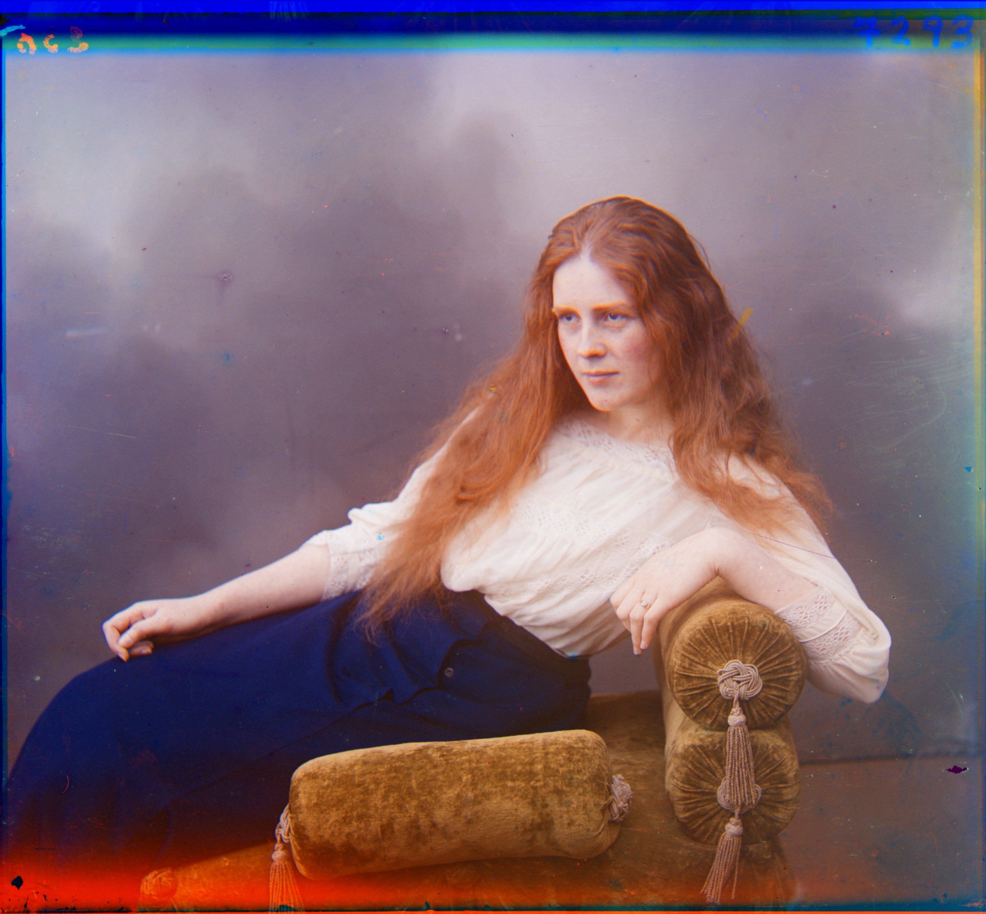
Displacement vectors (dx,dy): r:[8,54], b:[12,128]
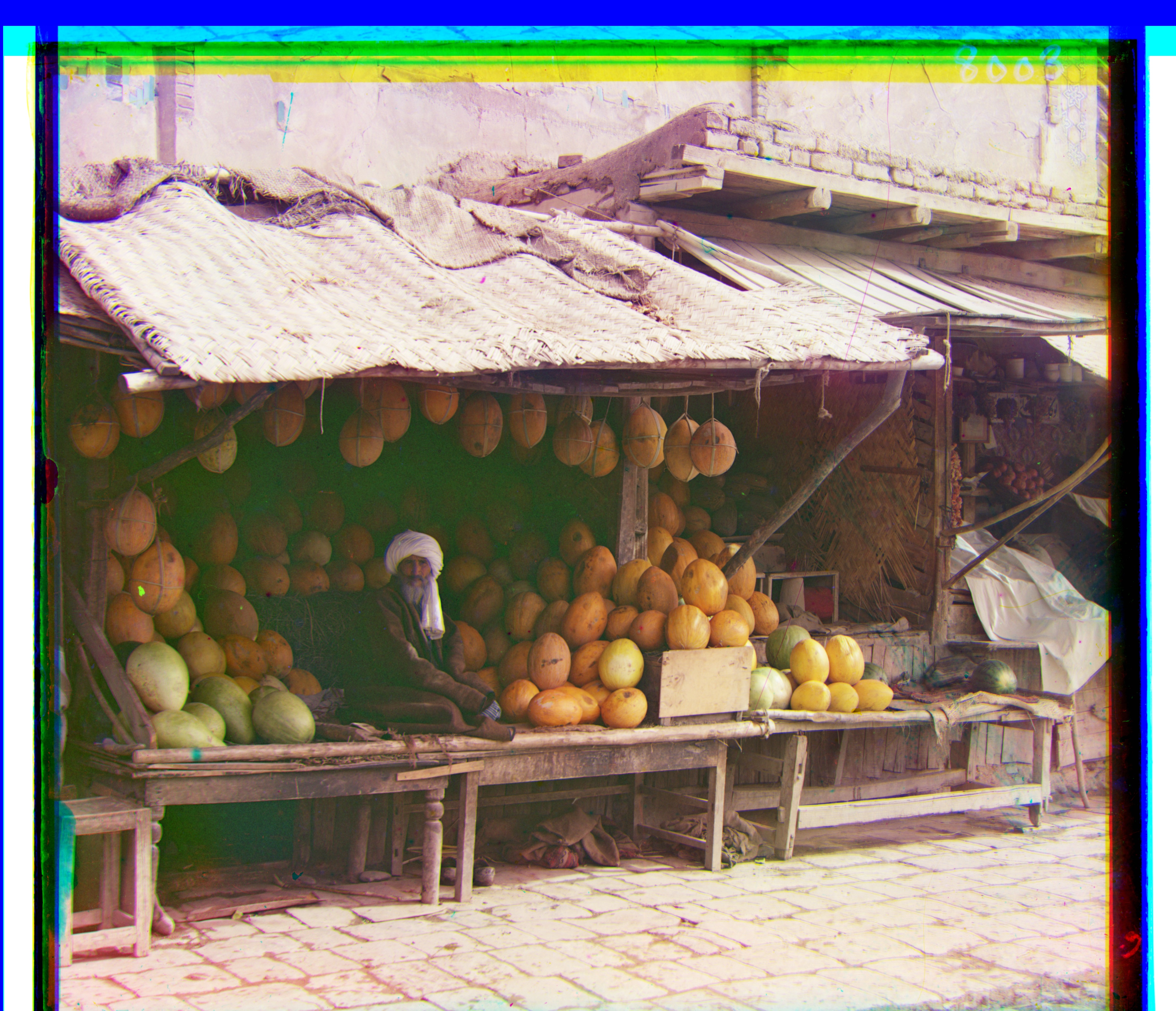
Displacement vectors (dx,dy): r:[10,83], b:[13,179]
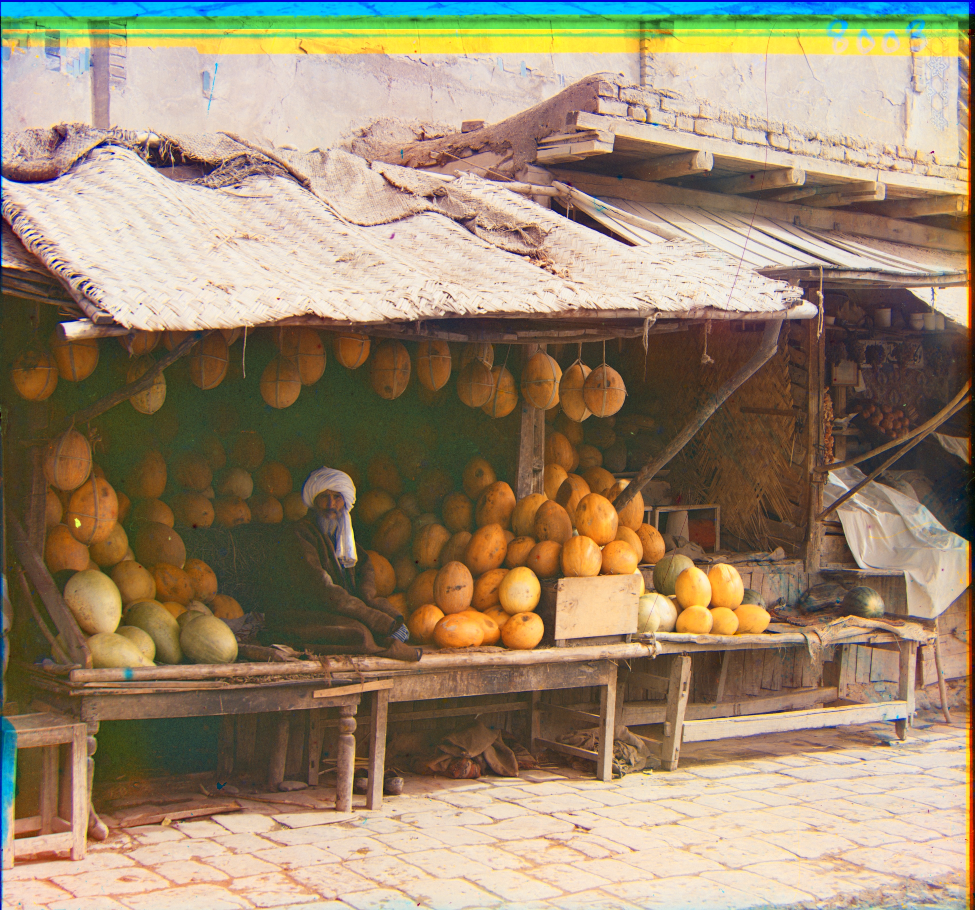
Displacement vectors (dx,dy): r:[10,83], b:[13,179]
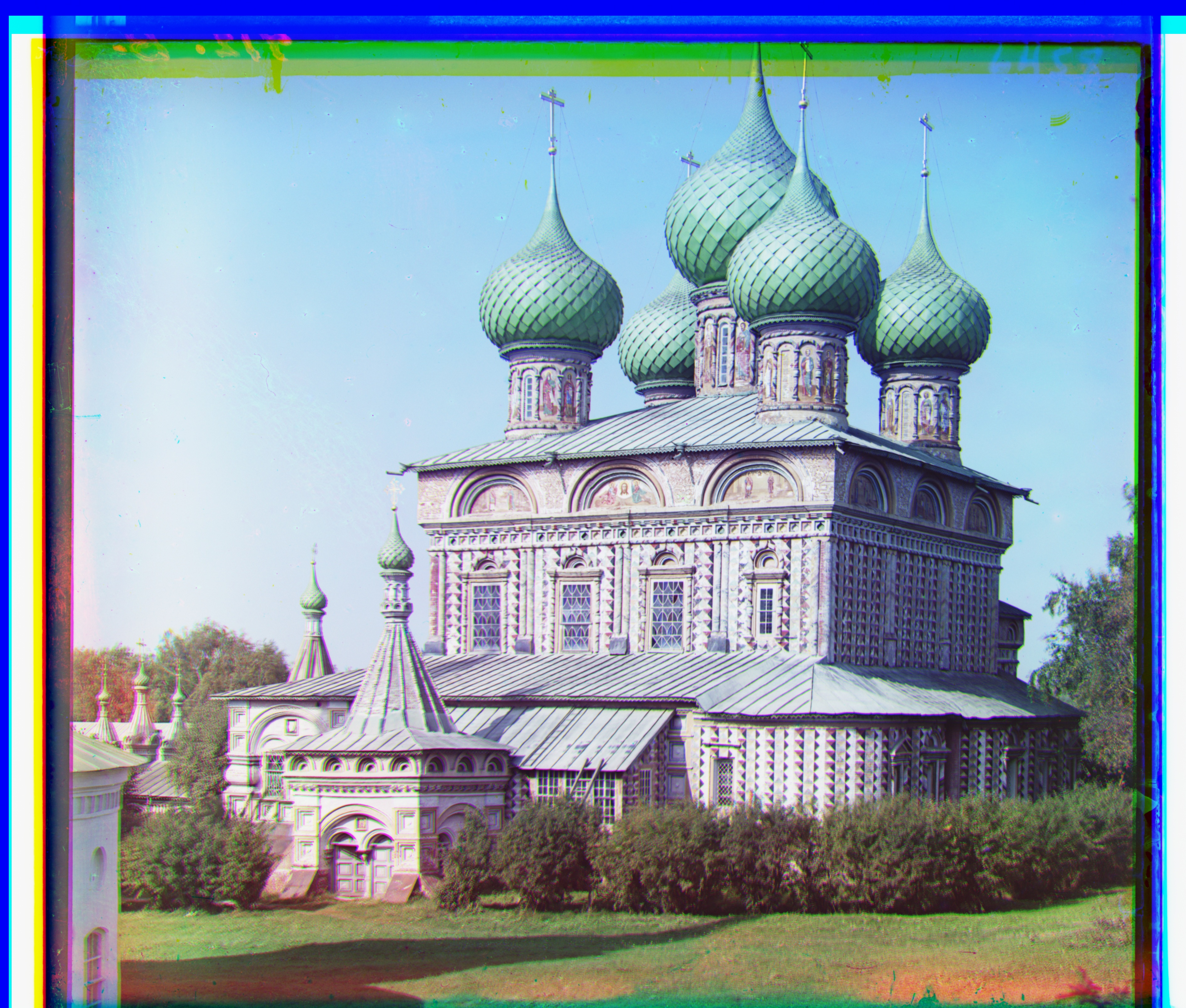
Displacement vectors (dx,dy): r:[28,50], b:[37,108]
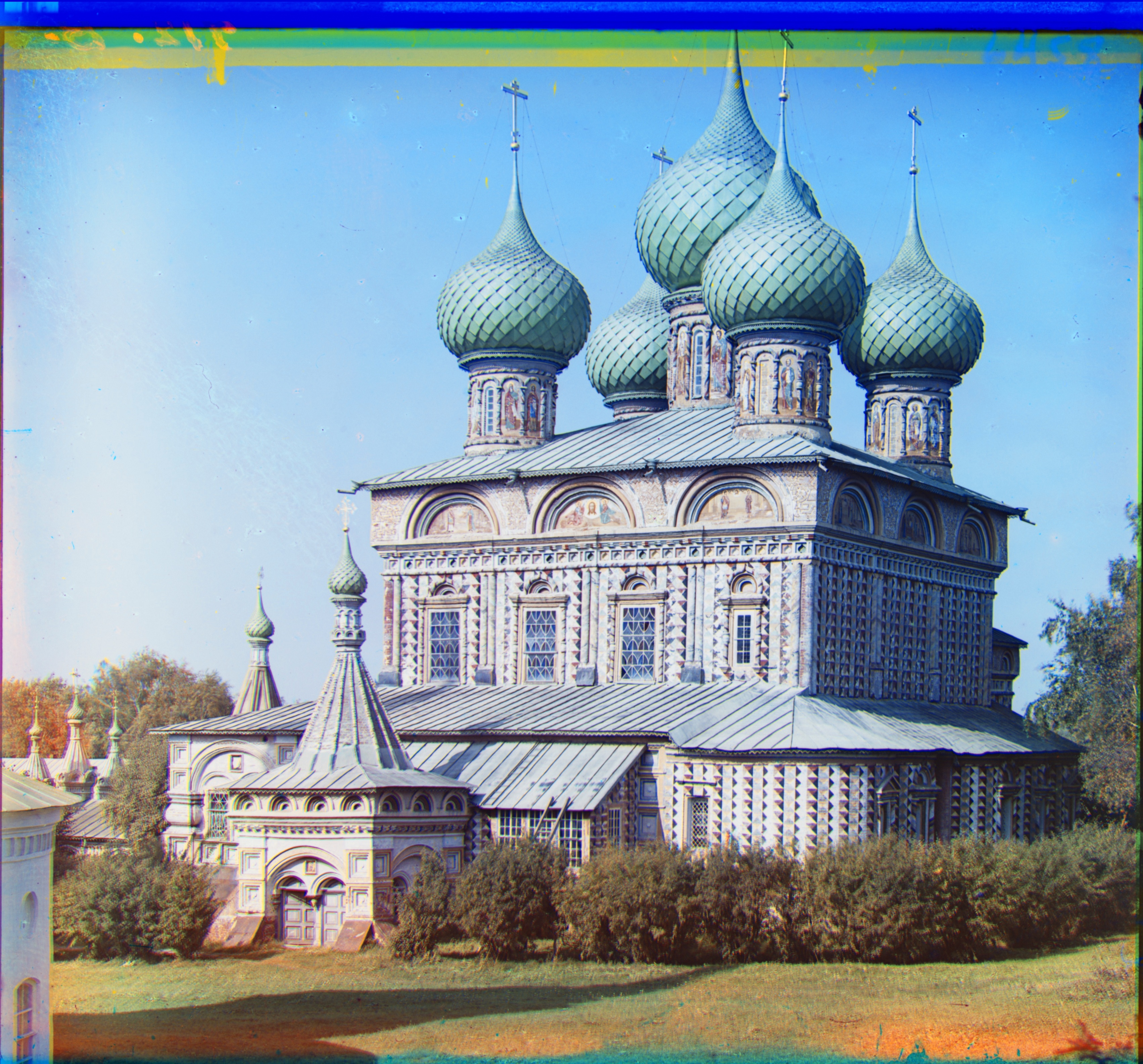
Displacement vectors (dx,dy): r:[28,50], b:[37,108]
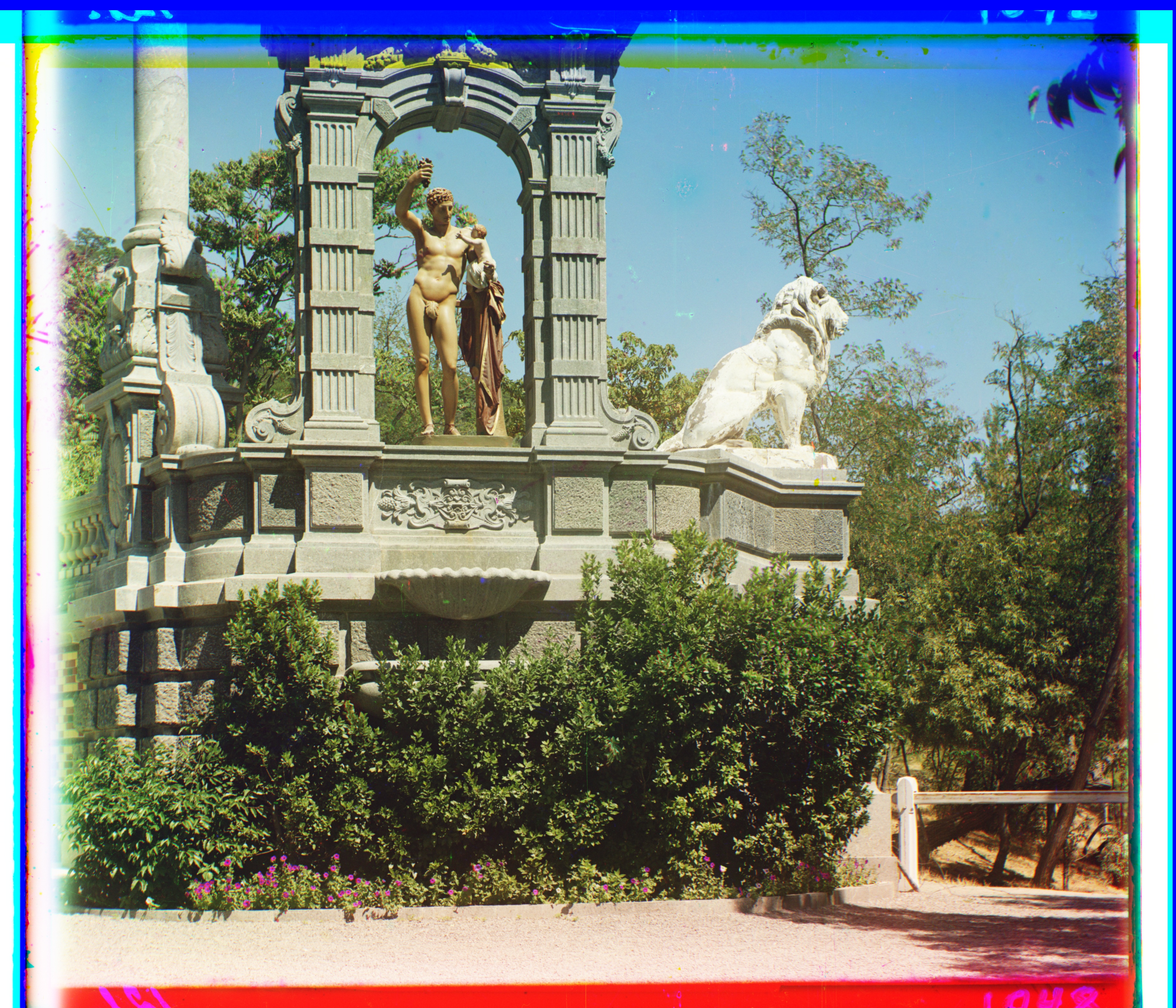
Displacement vectors (dx,dy): r:[-11,33], b:[-27,140]
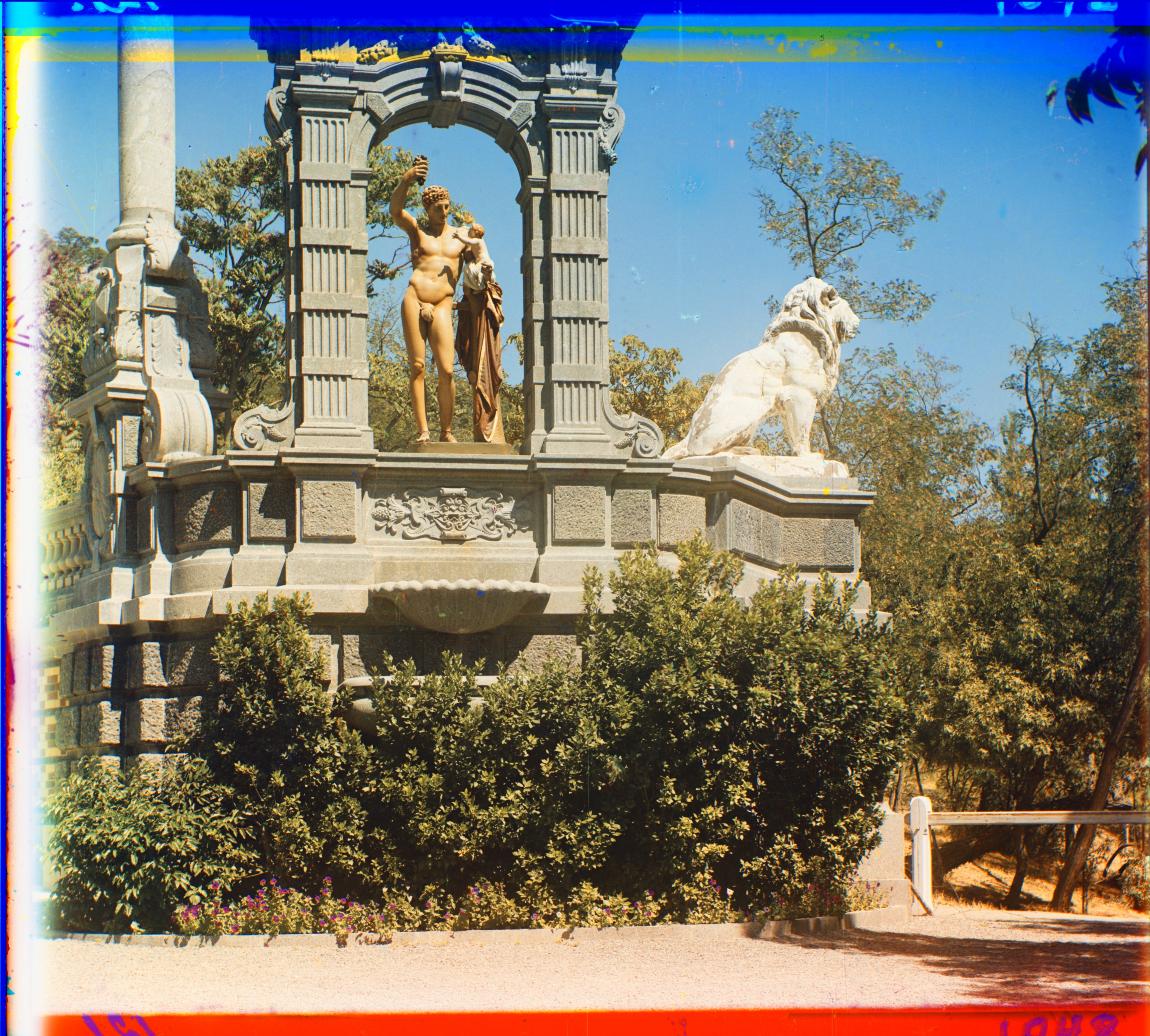
Displacement vectors (dx,dy): r:[-11,33], b:[-27,140]
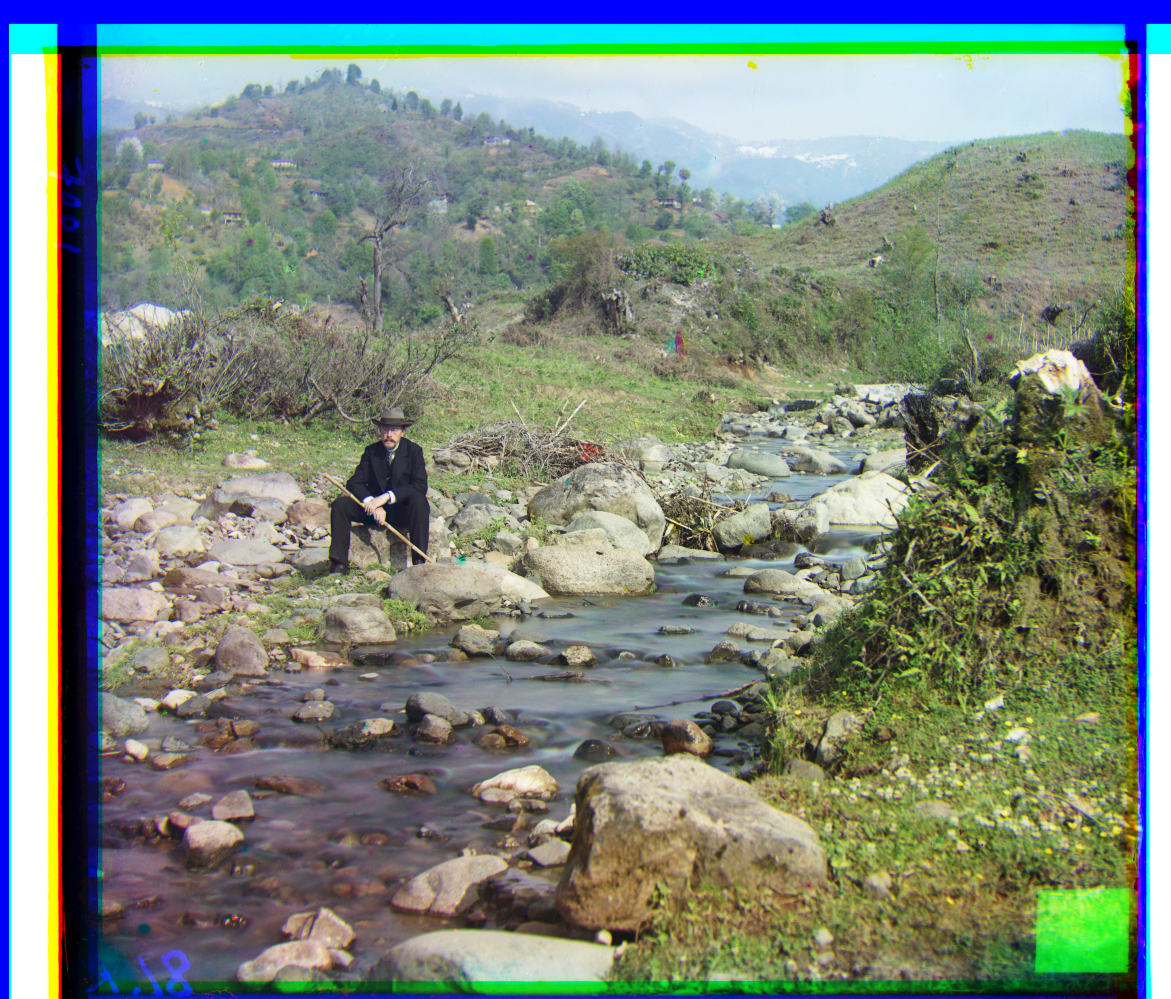
Displacement vectors (dx,dy): r:[29,77], b:[37,175]
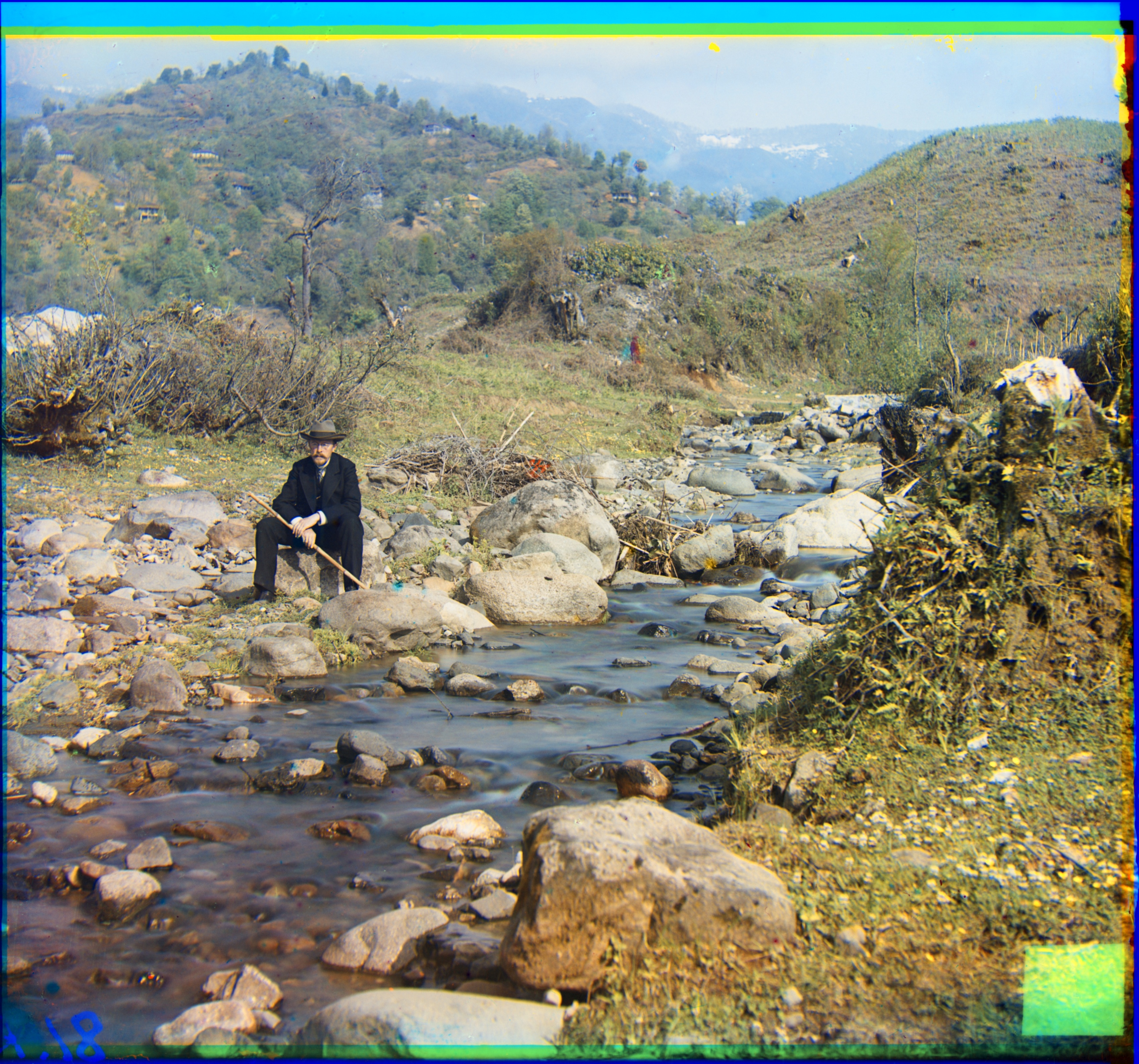
Displacement vectors (dx,dy): r:[29,77], b:[37,175]
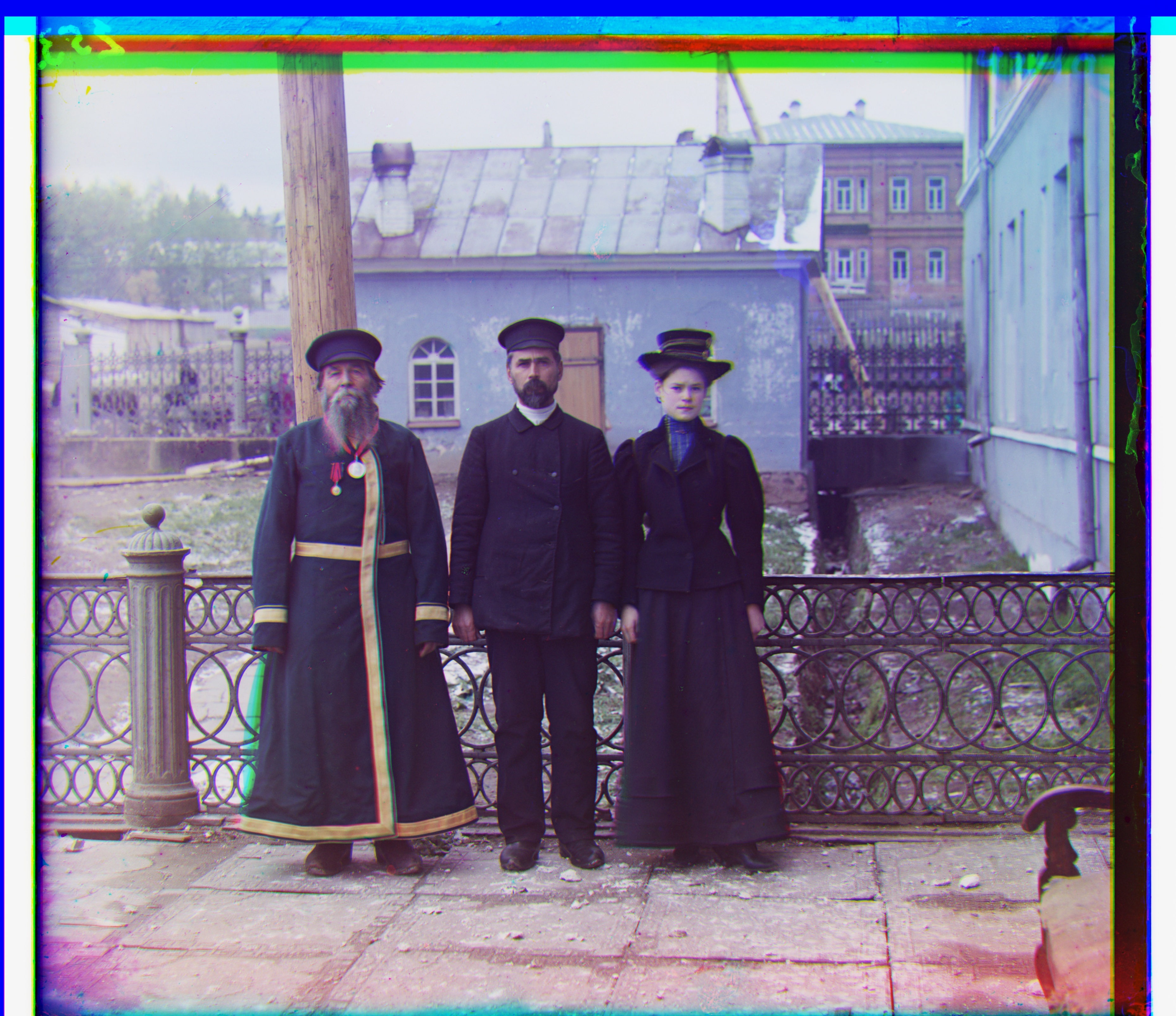
Displacement vectors (dx,dy): r:[14,52], b:[12,111]
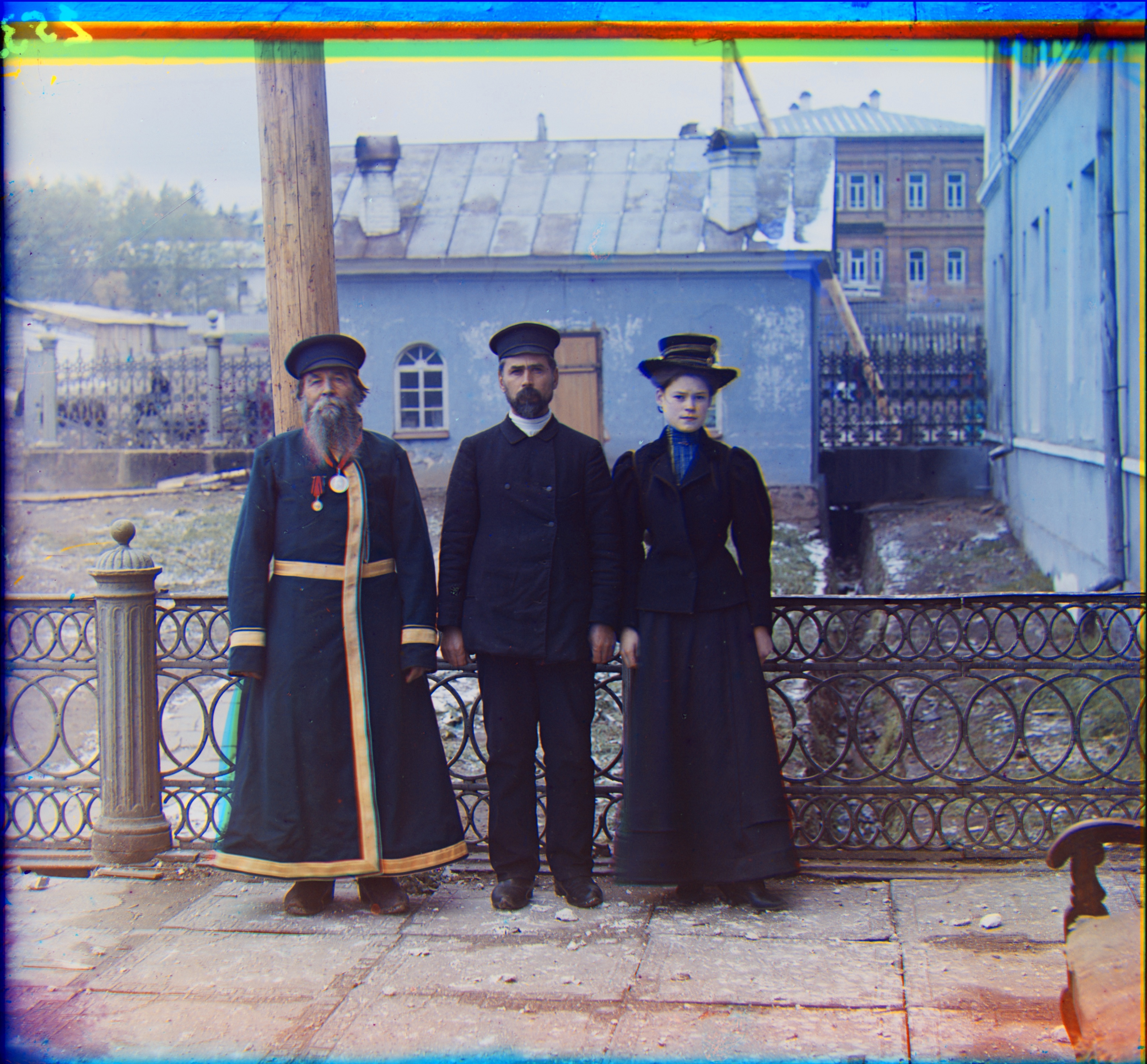
Displacement vectors (dx,dy): r:[14,52], b:[12,111]
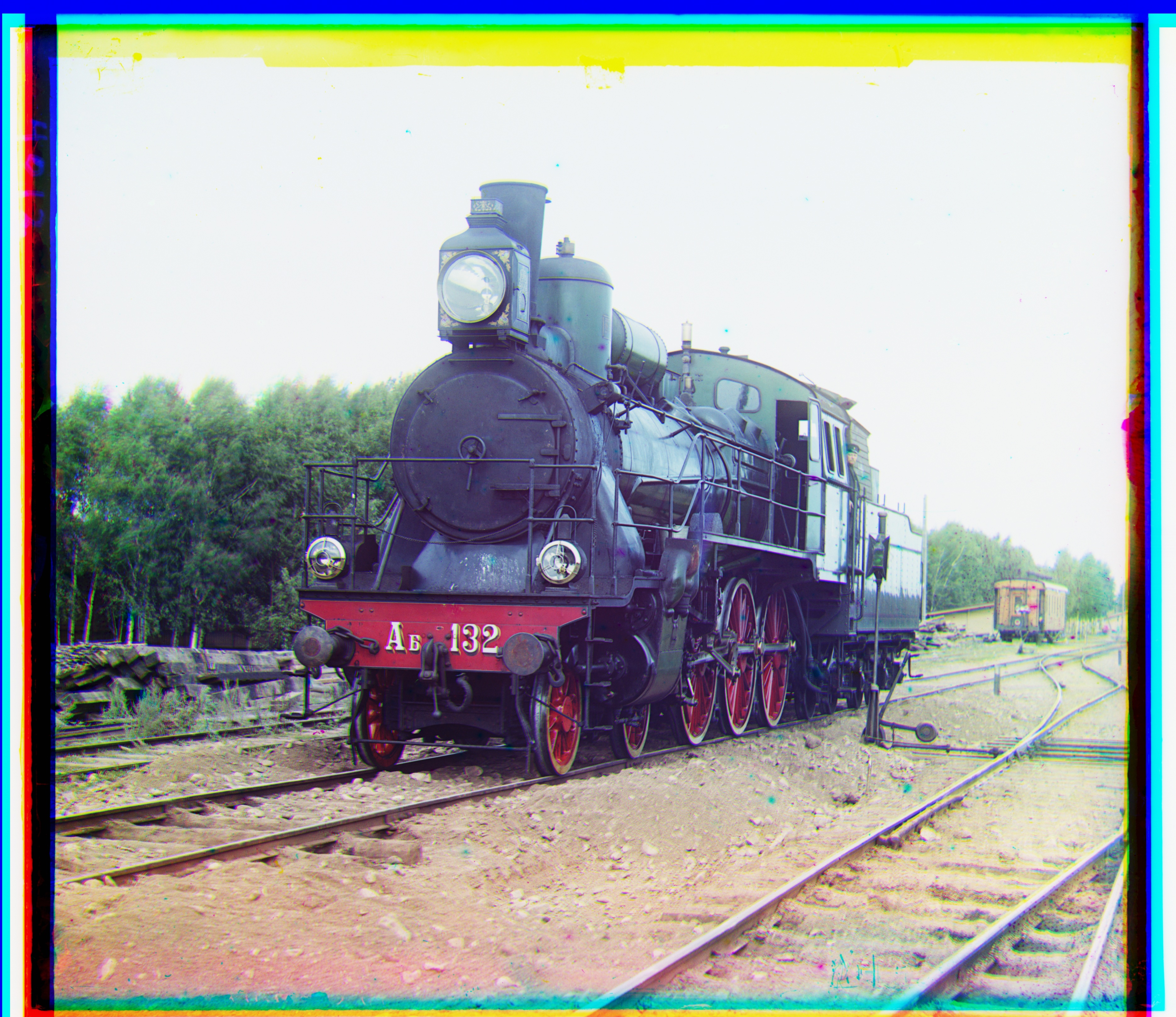
Displacement vectors (dx,dy): r:[7,43], b:[32,87]
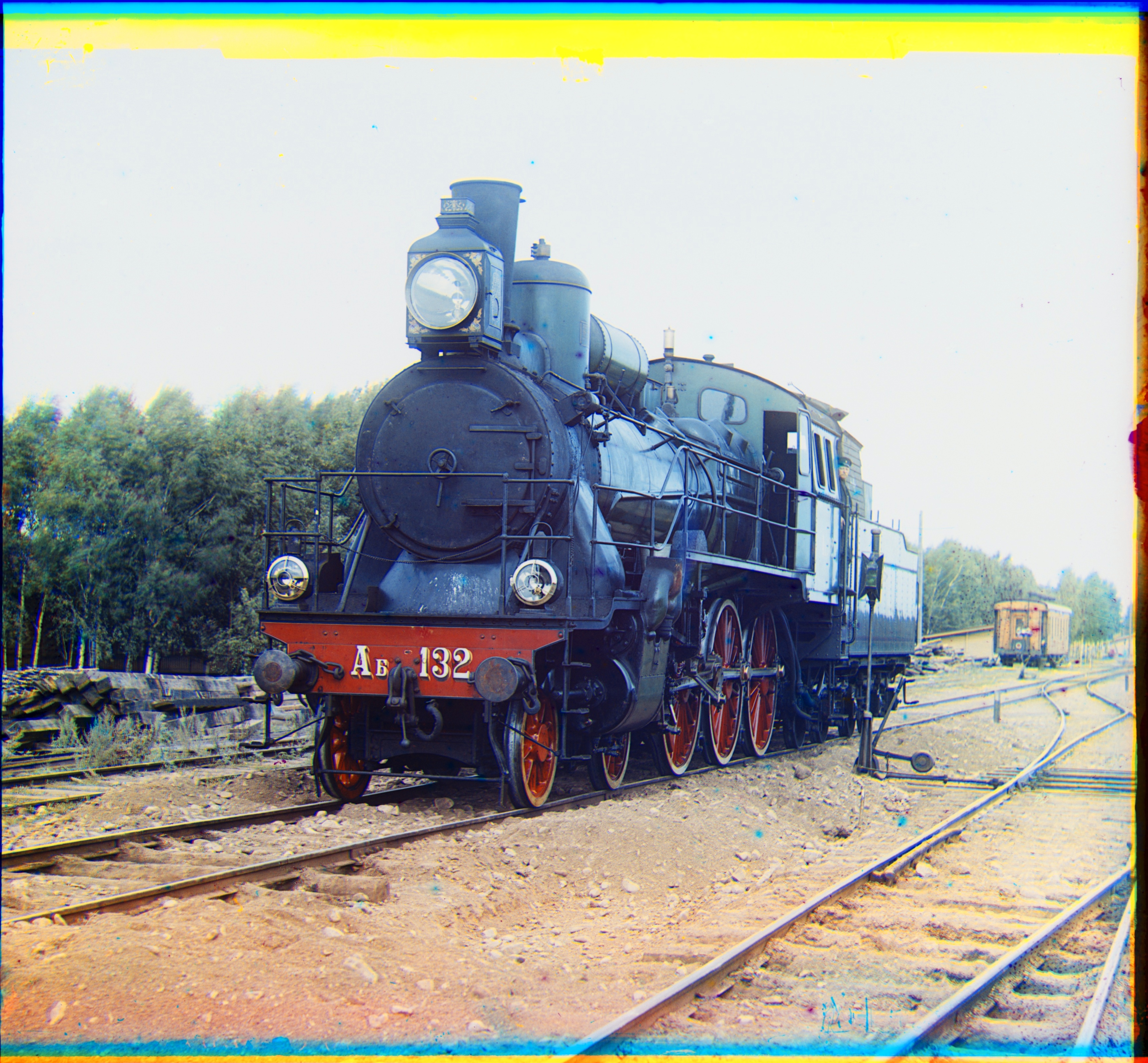
Displacement vectors (dx,dy): r:[7,43], b:[32,87]